Impulse Response Functions for a fitted steady-state BVAR model

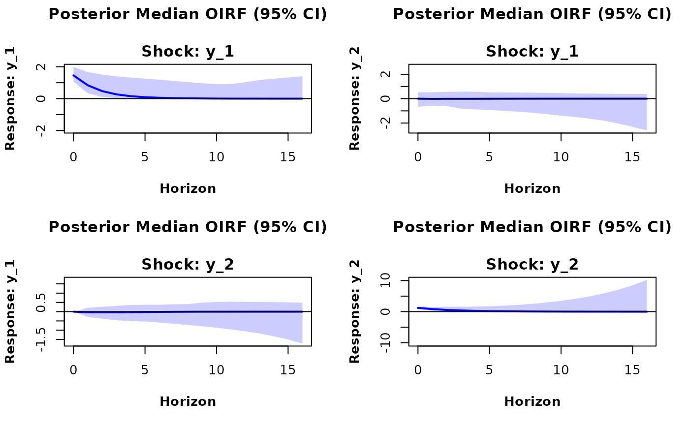
Computes and plots impulse response functions (IRFs) from a fitted steady-state bvar object. Supports both orthogonalized (OIRF) and generalized (GIRF) impulse responses, with optional conversion to annual growth rates.

Usage

IRF(
  x,
  H = 20,
  response = NULL,
  impulse = NULL,
  type = c("median", "mean"),
  method = c("OIRF", "GIRF"),
  ci = 0.95,
  t = NULL,
  growth_rate_idx = NULL
)

Arguments

x

A steady-state bvar object that has been passed through fit.

H

Integer. The forecast horizon for the IRF. Default 20.

response

Integer vector. Indices of the response variables to plot. If NULL (default), all responses are plotted.

impulse

Integer vector. Indices of the impulse variables to plot. If NULL (default), all impulses are plotted.

type

Character. Whether to use "median" or "mean" as the point estimate. Default "median".

method

Character. The IRF method: "OIRF" for orthogonalized or "GIRF" for generalized impulse responses. Default "OIRF".

ci

Numeric. The credible interval width. Default 0.95, i.e. 95%.

t

Integer. Time index for the covariance matrix when using stochastic volatility models. If NULL (default), the last time t is used.

growth_rate_idx

Integer vector. Indices of variables for which the impulse response is converted from a quarterly or monthly log first difference to an annual growth rate response, i.e. \(100 (\ln x_{t} - \ln x_{t-f})\), where \(f\) is the frequency of the data (4 for quarterly, 12 for monthly). Only suitable for variables specified as \(100 (\ln x_{t} - \ln x_{t-1})\), i.e. 100*diff(log(x)). Computed by summing up to \(f\) periods of the impulse response. Default is NULL.

Value

Invisibly returns a list with three arrays: the point estimate IRF, lower, and upper credible bounds, each of dimension k x k x (H+1).

Examples

# \donttest{
#homoscedastic with Jeffreys prior
yt <- matrix(rnorm(50), 25, 2)

bvar_obj <- bvar(data = yt)

bvar_obj <- setup(bvar_obj, p=1, deterministic = "constant")

bvar_obj <- priors(bvar_obj,
                   lambda_1 = 0.2,
                   lambda_2 = 0.5,
                   lambda_3 = 1,
                   first_own_lag_prior_mean = rep(1,2),
                   theta_Psi = rep(0, 2),
                   Omega_Psi = diag(0.1, 2, 2),
                   Jeffreys = TRUE,
                   SV = FALSE,
                   SV_type = NULL,
                   SV_priors = NULL)
                   
bvar_obj <- fit(bvar_obj,
                H = 8,
                iter = 200,
                warmup = 50,
                chains = 1,
                cores = 1)
#> ------------------------------------------------------------
#> Forecast horizon:
#> 8
#> 
#> Future deterministic variables (d_pred):
#>     constant
#> h=1        1
#> h=2        1
#> h=3        1
#> h=4        1
#> h=5        1
#> h=6        1
#> h=7        1
#> h=8        1
#> ------------------------------------------------------------
#> Estimating Stan model:
#> steady_state_bvar_homoscedastic_jeffreys_prior
#> 
#> Also generating draws from the joint predictive distribution
#> 
#> ...
#> 
#> SAMPLING FOR MODEL 'steady_state_bvar_homoscedastic_jeffreys_prior' NOW (CHAIN 1).
#> Chain 1: 
#> Chain 1: Gradient evaluation took 5.9e-05 seconds
#> Chain 1: 1000 transitions using 10 leapfrog steps per transition would take 0.59 seconds.
#> Chain 1: Adjust your expectations accordingly!
#> Chain 1: 
#> Chain 1: 
#> Chain 1: WARNING: There aren't enough warmup iterations to fit the
#> Chain 1:          three stages of adaptation as currently configured.
#> Chain 1:          Reducing each adaptation stage to 15%/75%/10% of
#> Chain 1:          the given number of warmup iterations:
#> Chain 1:            init_buffer = 7
#> Chain 1:            adapt_window = 38
#> Chain 1:            term_buffer = 5
#> Chain 1: 
#> Chain 1: Iteration:   1 / 200 [  0%]  (Warmup)
#> Chain 1: Iteration:  20 / 200 [ 10%]  (Warmup)
#> Chain 1: Iteration:  40 / 200 [ 20%]  (Warmup)
#> Chain 1: Iteration:  51 / 200 [ 25%]  (Sampling)
#> Chain 1: Iteration:  70 / 200 [ 35%]  (Sampling)
#> Chain 1: Iteration:  90 / 200 [ 45%]  (Sampling)
#> Chain 1: Iteration: 110 / 200 [ 55%]  (Sampling)
#> Chain 1: Iteration: 130 / 200 [ 65%]  (Sampling)
#> Chain 1: Iteration: 150 / 200 [ 75%]  (Sampling)
#> Chain 1: Iteration: 170 / 200 [ 85%]  (Sampling)
#> Chain 1: Iteration: 190 / 200 [ 95%]  (Sampling)
#> Chain 1: Iteration: 200 / 200 [100%]  (Sampling)
#> Chain 1: 
#> Chain 1:  Elapsed Time: 0.02 seconds (Warm-up)
#> Chain 1:                0.046 seconds (Sampling)
#> Chain 1:                0.066 seconds (Total)
#> Chain 1: 
#> Warning: Bulk Effective Samples Size (ESS) is too low, indicating posterior means and medians may be unreliable.
#> Running the chains for more iterations may help. See
#> https://mc-stan.org/misc/warnings.html#bulk-ess
#> Warning: Tail Effective Samples Size (ESS) is too low, indicating posterior variances and tail quantiles may be unreliable.
#> Running the chains for more iterations may help. See
#> https://mc-stan.org/misc/warnings.html#tail-ess
#> SAMPLING FINISHED
                
IRF(bvar_obj)

# }