Forecast from a fitted steady-state BVAR model

Computes and plots forecasts from a fitted bvar object. Draws from the joint predictive distribution are used to construct point forecasts and prediction intervals. Optionally converts monthly or quarterly growth rate forecasts to annual growth rates for selected variables.

Usage

forecast(
  x,
  pi = 0.95,
  fcst_type = c("mean", "median"),
  growth_rate_idx = NULL,
  plot_idx = NULL,
  show_all = FALSE
)

Arguments

x

A steady-state bvar object that has been passed through fit.

pi

Numeric. The prediction interval width. Default 0.95, i.e. 95% prediction interval.

fcst_type

Character. Whether to use "mean" or "median" as the point forecast. Default "mean".

growth_rate_idx

Integer vector. Indices of variables of which to convert forecasts to annual growth rates \(\ln x_{t} - \ln x_{t-f}\), where \(f\) is the frequency of the data (4 for quarterly, 12 for monthly). Only suitable for variables specified as \(\ln x_{t} - \ln x_{t-1}\), i.e. diff(log(x)) or 100*diff(log(x)). Computed by summing up to \(f\) log first differences. Default is NULL.

plot_idx

Integer vector. Indices of variables to plot. If NULL (default), all variables are plotted. Forecasts are always computed and returned for all variables, regardless of plot_idx.

show_all

Logical. If FALSE (default), only the last two years of history are shown alongside the forecast. If TRUE, the full history is shown.

Value

Invisibly returns a list with three matrices: forecast, lower, and upper, each of dimension H x k where H is the forecast horizon and k is the number of variables.

Examples

# \donttest{
#homoscedastic with Jeffreys prior
yt <- matrix(rnorm(50), 25, 2)

bvar_obj <- bvar(data = yt)

bvar_obj <- setup(bvar_obj, p=1, deterministic = "constant")

bvar_obj <- priors(bvar_obj,
                   lambda_1 = 0.2,
                   lambda_2 = 0.5,
                   lambda_3 = 1,
                   first_own_lag_prior_mean = rep(1,2),
                   theta_Psi = rep(0, 2),
                   Omega_Psi = diag(0.1, 2, 2),
                   Jeffreys = TRUE,
                   SV = FALSE,
                   SV_type = NULL,
                   SV_priors = NULL)
                   
bvar_obj <- fit(bvar_obj,
                H = 8,
                d_pred = matrix(rep(1,8)),
                iter = 200,
                warmup = 50,
                chains = 1,
                cores = 1)
#> 
#> SAMPLING FOR MODEL 'steady_state_bvar_homoscedastic_jeffreys_prior' NOW (CHAIN 1).
#> Chain 1: 
#> Chain 1: Gradient evaluation took 7.4e-05 seconds
#> Chain 1: 1000 transitions using 10 leapfrog steps per transition would take 0.74 seconds.
#> Chain 1: Adjust your expectations accordingly!
#> Chain 1: 
#> Chain 1: 
#> Chain 1: WARNING: There aren't enough warmup iterations to fit the
#> Chain 1:          three stages of adaptation as currently configured.
#> Chain 1:          Reducing each adaptation stage to 15%/75%/10% of
#> Chain 1:          the given number of warmup iterations:
#> Chain 1:            init_buffer = 7
#> Chain 1:            adapt_window = 38
#> Chain 1:            term_buffer = 5
#> Chain 1: 
#> Chain 1: Iteration:   1 / 200 [  0%]  (Warmup)
#> Chain 1: Iteration:  20 / 200 [ 10%]  (Warmup)
#> Chain 1: Iteration:  40 / 200 [ 20%]  (Warmup)
#> Chain 1: Iteration:  51 / 200 [ 25%]  (Sampling)
#> Chain 1: Iteration:  70 / 200 [ 35%]  (Sampling)
#> Chain 1: Iteration:  90 / 200 [ 45%]  (Sampling)
#> Chain 1: Iteration: 110 / 200 [ 55%]  (Sampling)
#> Chain 1: Iteration: 130 / 200 [ 65%]  (Sampling)
#> Chain 1: Iteration: 150 / 200 [ 75%]  (Sampling)
#> Chain 1: Iteration: 170 / 200 [ 85%]  (Sampling)
#> Chain 1: Iteration: 190 / 200 [ 95%]  (Sampling)
#> Chain 1: Iteration: 200 / 200 [100%]  (Sampling)
#> Chain 1: 
#> Chain 1:  Elapsed Time: 0.026 seconds (Warm-up)
#> Chain 1:                0.08 seconds (Sampling)
#> Chain 1:                0.106 seconds (Total)
#> Chain 1: 
#> Warning: The largest R-hat is 1.08, indicating chains have not mixed.
#> Running the chains for more iterations may help. See
#> https://mc-stan.org/misc/warnings.html#r-hat
#> Warning: Bulk Effective Samples Size (ESS) is too low, indicating posterior means and medians may be unreliable.
#> Running the chains for more iterations may help. See
#> https://mc-stan.org/misc/warnings.html#bulk-ess
#> Warning: Tail Effective Samples Size (ESS) is too low, indicating posterior variances and tail quantiles may be unreliable.
#> Running the chains for more iterations may help. See
#> https://mc-stan.org/misc/warnings.html#tail-ess

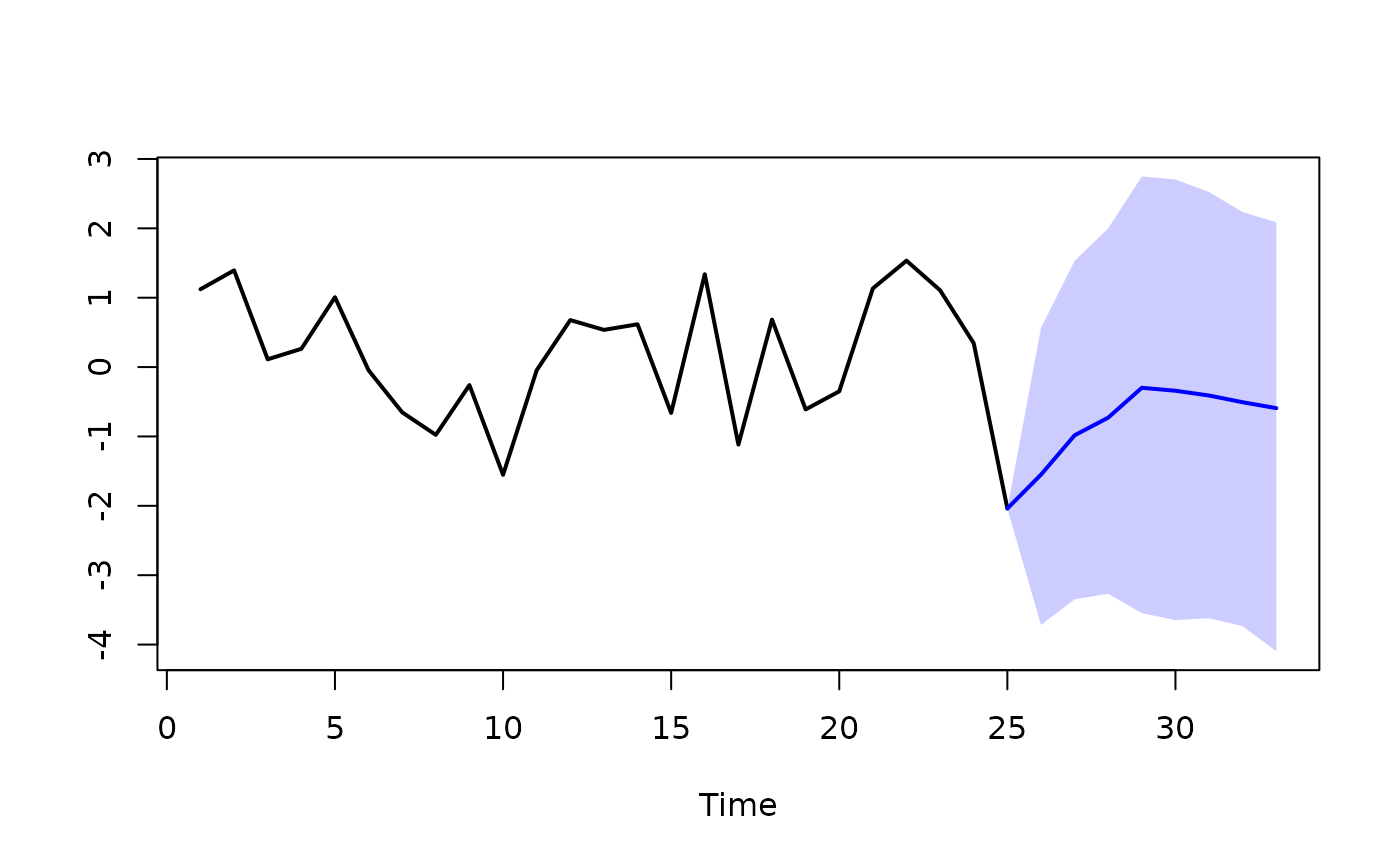
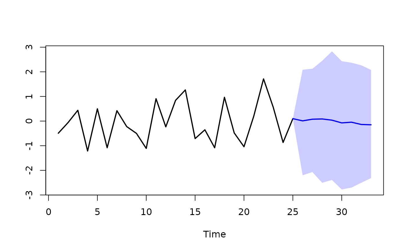
(fcst <- forecast(bvar_obj, pi = 0.90, show_all = TRUE))


#> $forecast
#>            [,1]         [,2]
#> [1,] -1.5507742  0.009340416
#> [2,] -0.9838015  0.075657629
#> [3,] -0.7285100  0.086311839
#> [4,] -0.2984426  0.037254121
#> [5,] -0.3410332 -0.073507585
#> [6,] -0.4102036 -0.045218146
#> [7,] -0.5068994 -0.137687275
#> [8,] -0.5921016 -0.150132450
#> 
#> $lower
#>           [,1]      [,2]
#> [1,] -3.717534 -2.199458
#> [2,] -3.347816 -2.069477
#> [3,] -3.266988 -2.503793
#> [4,] -3.546320 -2.391206
#> [5,] -3.647156 -2.777127
#> [6,] -3.619673 -2.700129
#> [7,] -3.735963 -2.504099
#> [8,] -4.095228 -2.313835
#> 
#> $upper
#>           [,1]     [,2]
#> [1,] 0.5650957 2.083305
#> [2,] 1.5304052 2.124948
#> [3,] 1.9997609 2.445404
#> [4,] 2.7482622 2.831531
#> [5,] 2.7041119 2.432656
#> [6,] 2.5230543 2.368828
#> [7,] 2.2344466 2.264161
#> [8,] 2.0876712 2.077583
#> 
# }