Plot steady-state priors

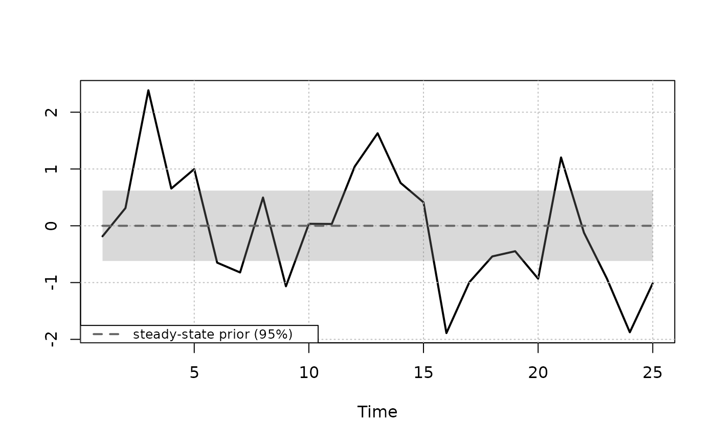
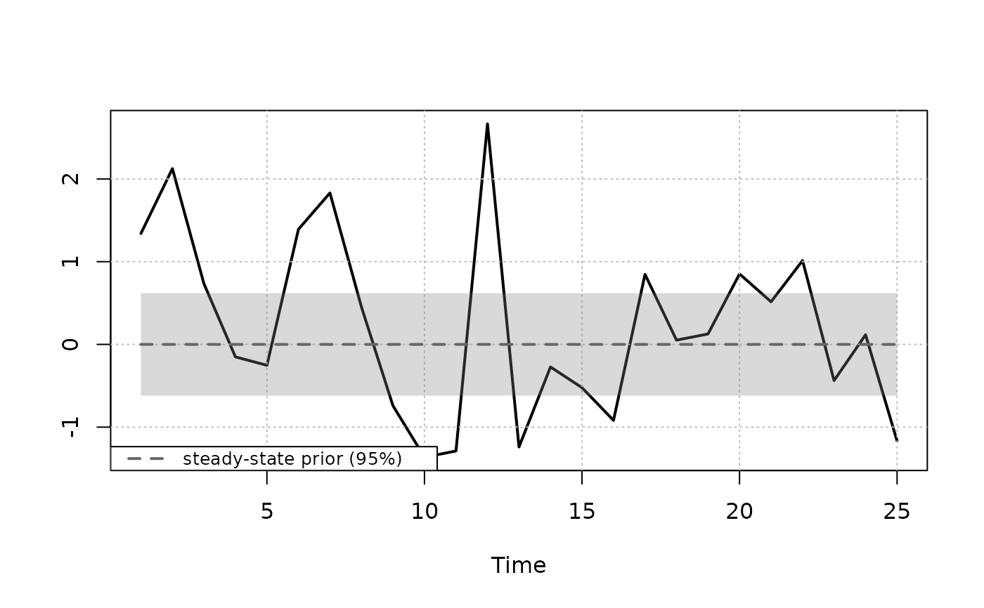
Produces time series plots of the data along with the implied prior for the steady state \(\mu_t = \Psi d_t\).

Usage

steady_state_priors_plot(
  x,
  interval = 0.95,
  growth_rate_idx = NULL,
  plot_idx = NULL
)

Arguments

x

A steady-state bvar object that has been passed through priors.

interval

Numeric. The prior interval width. Default 0.95, i.e. a 95% prior interval for the steady state.

growth_rate_idx

Integer vector. Indices of variables specified as \(100 (\ln x_{t} - \ln x_{t-1})\), i.e. 100*diff(log(x)), for which the historical series is converted to year-over-year (annual) growth scale \(100 (\ln x_{t} - \ln x_{t-f})\) and the steady-state prior is converted to the annualized (not annual) growth scale \(f100(\ln x_{t} - \ln x_{t-1})\) where \(f\) = frequency. Default is NULL.

plot_idx

Integer vector. Indices of variables to plot. If NULL (default), all variables are plotted.

Value

Invisibly returns a list with three matrices, lower, mean, and upper, each of dimension T x k giving the steady-state prior bounds and mean over the historical sample. For growth_rate_idx columns, these are on the annualized scale.

Details

The implied prior for the steady state \(\mu_t = \Psi d_t\) is based on the prior for \(\Psi\)

$$\mathrm{vec}(\Psi) \sim \mathrm{N}(\theta_\Psi, \Omega_\Psi)$$

which is specified in priors. Note that it is assumed that \(\Omega_\Psi\) is diagonal.

Examples

# \donttest{
yt <- matrix(rnorm(50), 25, 2)

bvar_obj <- bvar(data = yt)

bvar_obj <- setup(bvar_obj, p = 1, deterministic = "constant")

bvar_obj <- priors(bvar_obj,
                   lambda_1 = 0.2,
                   lambda_2 = 0.5,
                   lambda_3 = 1,
                   first_own_lag_prior_mean = rep(1, 2),
                   theta_Psi = rep(0, 2),
                   Omega_Psi = diag(0.1, 2, 2),
                   Jeffreys = TRUE)

steady_state_priors_plot(bvar_obj)


# }