Plot stochastic volatility estimates and forecasts

Produces time series plots of posterior stochastic volatility estimates over the estimation sample together with predictive paths over the forecast horizon for a fitted steady-state bvar object with stochastic volatility.

Usage

stochastic_volatility_plot(
  x,
  ci = 0.95,
  vol = "log_lambda",
  stat = "mean",
  plot_idx = NULL,
  xlim = NULL,
  ylim = NULL
)

Arguments

x

A steady-state bvar object that has been passed through fit with stochastic volatility enabled.

ci

Numeric. Interval level. Default is 0.95.

vol

Character. Volatility representation: "log_lambda" (default) or "sd".

stat

Character. Posterior summary statistic to use as point estimate: "mean" (default) or "median".

plot_idx

Integer vector. Indices of variables to plot. If NULL (default), all variables are plotted.

xlim

Numeric vector of length 2. Optional x-axis limits.

ylim

Numeric vector of length 2. Optional y-axis limits.

Value

An invisible list with:

• estimated: List of posterior summaries for the estimation sample:

  • point: \(T \times k\) matrix of posterior point estimates (mean or median depending on stat)

  • lower: \(T \times k\) matrix of lower credible bounds

  • upper: \(T \times k\) matrix of upper credible bounds

• predicted: List of posterior summaries for the forecast horizon:

  • point: \((T+H) \times k\) matrix of predictive point estimates (mean or median depending on stat)

  • lower: \((T+H) \times k\) matrix of lower bound of prediction interval

  • upper: \((T+H) \times k\) matrix of upper bound of prediction interval

Details

The function supports two volatility representations:

• "log_lambda": log variances

• "sd": implied standard deviations

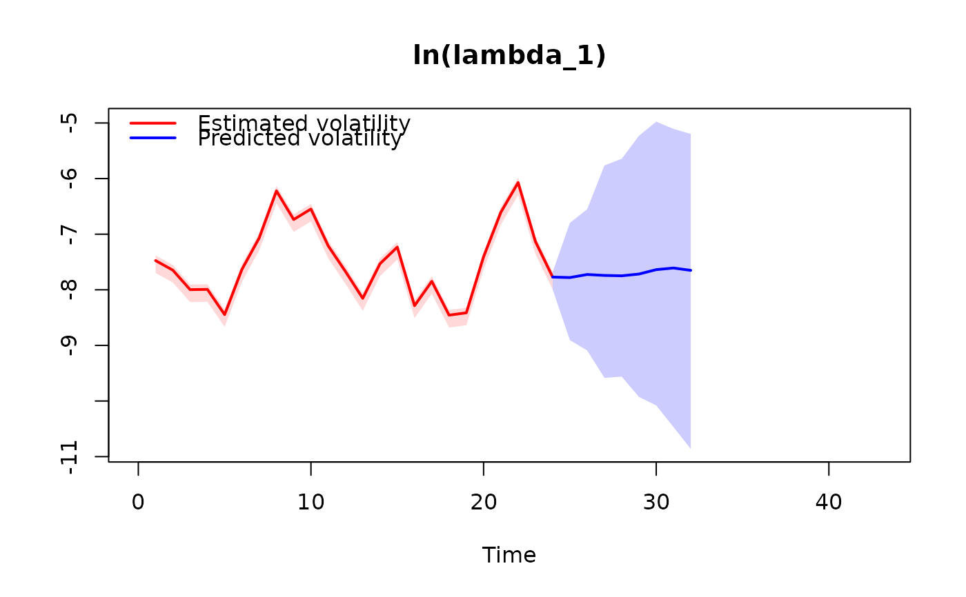
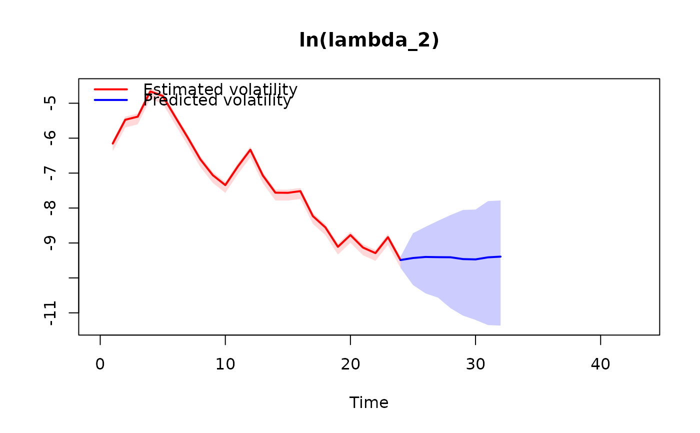
For each selected variable, the function plots the posterior point estimate path and credible bands over the estimation sample, and the predictive point estimate path and prediction intervals over the forecast horizon.

Examples

# \donttest{
yt <- matrix(rnorm(50), 25, 2)

bvar_obj <- bvar(data = yt)

bvar_obj <- setup(bvar_obj, p = 1, deterministic = "constant")

k <- bvar_obj$setup$k
n_free_params_A <- bvar_obj$setup$n_free_params_A

SV_priors <- list(
theta_A             =  rep(0, n_free_params_A),
Omega_A             =  diag(1000, n_free_params_A),
mu_log_lambda_1     =  rep(0, k),
sigma2_log_lambda_1 =  rep(1000, k),
alpha_phi           =  rep(5, k),
beta_phi            = (rep(5, k) - 1) * rep(0.1, k)
)

bvar_obj <- priors(bvar_obj,
                   theta_Psi = rep(0, 2),
                   Omega_Psi = diag(0.1, 2, 2),
                   SV = TRUE,
                   SV_type = "RW",
                   SV_priors = SV_priors)

bvar_obj <- fit(bvar_obj,
                H = 8,
                d_pred = matrix(rep(1, 8)),
                iter = 200,
                warmup = 50,
                chains = 1,
                cores = 1,
                verbose = FALSE)
#> 
#> SAMPLING FOR MODEL 'steady_state_bvar_RW_stochastic_volatility' NOW (CHAIN 1).
#> Chain 1: 
#> Chain 1: Gradient evaluation took 0.000145 seconds
#> Chain 1: 1000 transitions using 10 leapfrog steps per transition would take 1.45 seconds.
#> Chain 1: Adjust your expectations accordingly!
#> Chain 1: 
#> Chain 1: 
#> Chain 1: WARNING: There aren't enough warmup iterations to fit the
#> Chain 1:          three stages of adaptation as currently configured.
#> Chain 1:          Reducing each adaptation stage to 15%/75%/10% of
#> Chain 1:          the given number of warmup iterations:
#> Chain 1:            init_buffer = 7
#> Chain 1:            adapt_window = 38
#> Chain 1:            term_buffer = 5
#> Chain 1: 
#> Chain 1: Iteration:   1 / 200 [  0%]  (Warmup)
#> Chain 1: Iteration:  20 / 200 [ 10%]  (Warmup)
#> Chain 1: Iteration:  40 / 200 [ 20%]  (Warmup)
#> Chain 1: Iteration:  51 / 200 [ 25%]  (Sampling)
#> Chain 1: Iteration:  70 / 200 [ 35%]  (Sampling)
#> Chain 1: Iteration:  90 / 200 [ 45%]  (Sampling)
#> Chain 1: Iteration: 110 / 200 [ 55%]  (Sampling)
#> Chain 1: Iteration: 130 / 200 [ 65%]  (Sampling)
#> Chain 1: Iteration: 150 / 200 [ 75%]  (Sampling)
#> Chain 1: Iteration: 170 / 200 [ 85%]  (Sampling)
#> Chain 1: Iteration: 190 / 200 [ 95%]  (Sampling)
#> Chain 1: Iteration: 200 / 200 [100%]  (Sampling)
#> Chain 1: 
#> Chain 1:  Elapsed Time: 0.034 seconds (Warm-up)
#> Chain 1:                1.869 seconds (Sampling)
#> Chain 1:                1.903 seconds (Total)
#> Chain 1: 
#> Warning: There were 1 transitions after warmup that exceeded the maximum treedepth. Increase max_treedepth above 10. See
#> https://mc-stan.org/misc/warnings.html#maximum-treedepth-exceeded
#> Warning: There were 1 chains where the estimated Bayesian Fraction of Missing Information was low. See
#> https://mc-stan.org/misc/warnings.html#bfmi-low
#> Warning: Examine the pairs() plot to diagnose sampling problems
#> Warning: The largest R-hat is NA, indicating chains have not mixed.
#> Running the chains for more iterations may help. See
#> https://mc-stan.org/misc/warnings.html#r-hat
#> Warning: Bulk Effective Samples Size (ESS) is too low, indicating posterior means and medians may be unreliable.
#> Running the chains for more iterations may help. See
#> https://mc-stan.org/misc/warnings.html#bulk-ess
#> Warning: Tail Effective Samples Size (ESS) is too low, indicating posterior variances and tail quantiles may be unreliable.
#> Running the chains for more iterations may help. See
#> https://mc-stan.org/misc/warnings.html#tail-ess

stochastic_volatility_plot(bvar_obj, ci = 0.95)


# }